
Motivation
Enterprise grade hardware (including Graphical Processing Units) for Artificial Intelligence operations are scarce. Significant effort and capital seek to expand access. However, even when access expands significantly, a variety of use cases will constrain AI activities to less powerful hardware. For example:
- Development and test environments must be available to each individual AI developer and cannot rely on expensive powerful hardware. Such environments validate correctness of, among other things, 1) ultimate training at scale and 2) inference in production.
- Smaller companies, startups, individual researchers, individual creators and even resource-constrained labs within larger organizations will lack funds needed to gain access to enterprise-grade software.
In this blog, we detail one method for conducting inference using hardware too small to hold the entirety of an AI model. Several techniques exist to solve this problem, including quantization, model shards, device offloading, and decoupled pipelines. This blog will focus on decoupled pipelines and briefly touch device offloading. (We don't treat model training. Look out for a future blog post.)
(See the accompanying notebook on github for full code and additional details.)
Conceptual Approach
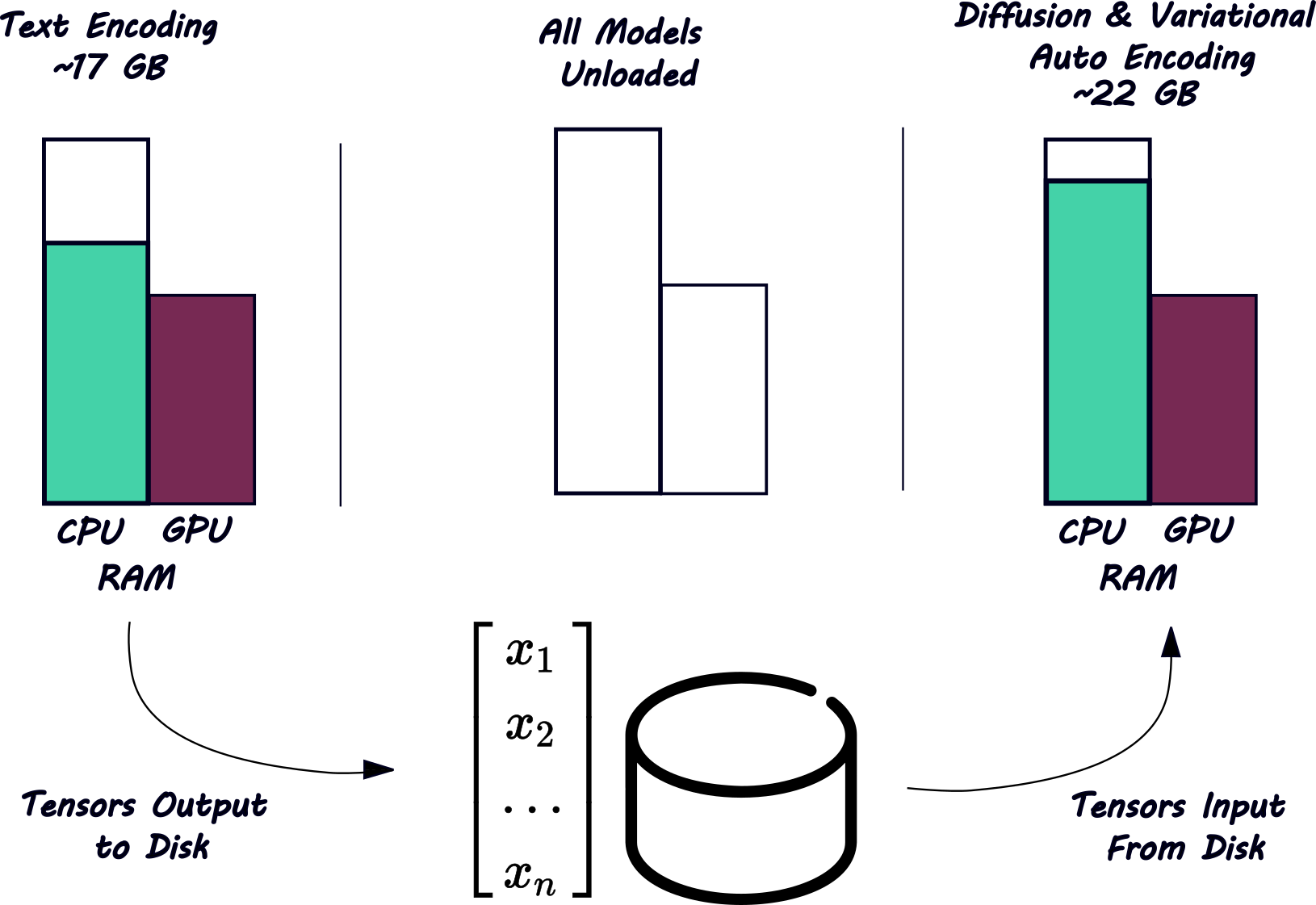
Rather than load all required models into memory and keep them there throughout processing, we'll load only the models we need to produce the next step. Then we'll unload those models before loading the new ones—a Decoupled Pipeline.
We'll use 8 GB of GPU RAM (VRAM) and 30 GB of CPU RAM to infer from a model whose native 32-bit float precision occupies over 61 GB. (Note that our actual hardware is significantly larger than that—12 GB of VRAM and 48 GB of RAM—to allow for the overhead of the operating system, CUDA, and PyTorch, which is significantly smaller than enterprise servers and accessible to consumers.)
We'll use the Flux text to image pipeline, in part because loading all its models in native precision requires 61 GB, well above our targeted hardware capacity.
As with most AI models, Flux uses a pipeline of multiple steps to process from text prompt to image.
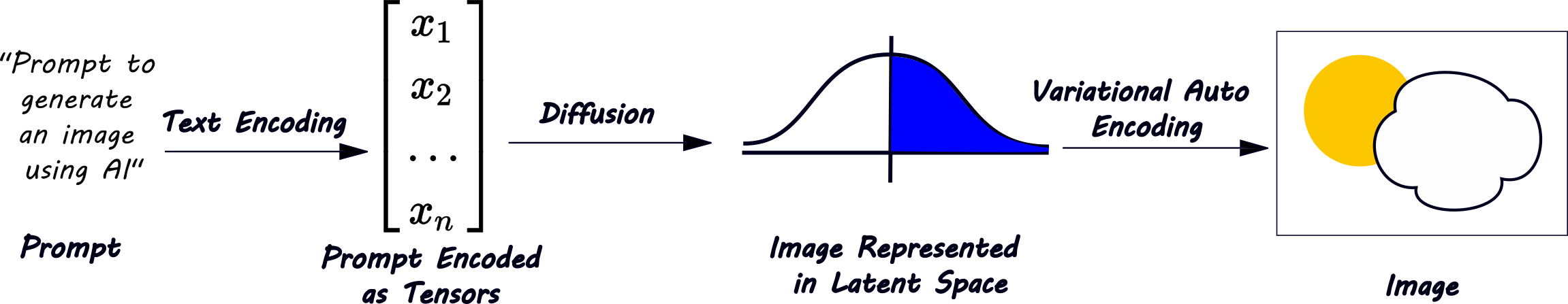
We'll decouple this pipeline as shown below. Note that while loading all models simultaneously would lead to out of memory errors, loading them a few at a time allows the pipeline to run.
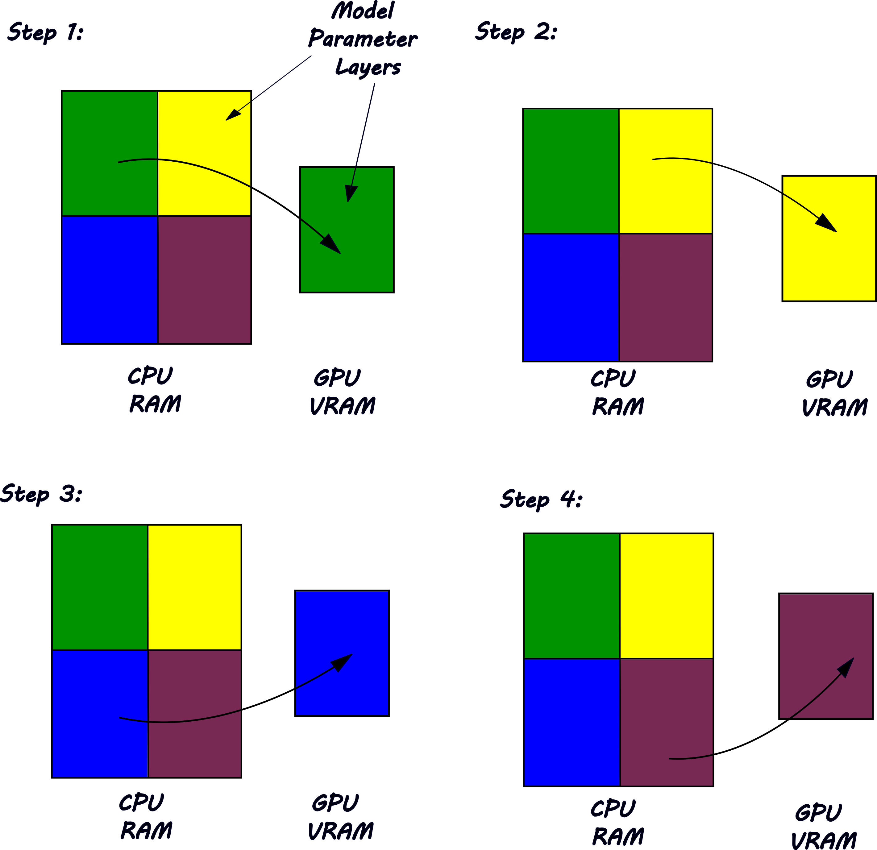
So far so good. But if we want a reasonable time to inference for either model, we don't want our CPU to do much computation because CPUs lack optimization for parallel matrix operations that AI models demand. Our GPU can't operate efficiently if it must constantly call to CPU RAM to get the data it needs, so model parameters should reside in VRAM—which we don't have enough of—as much as possible. HuggingFace Accelerate provides an solution here too. Accelerate's Big Model Inference leverages Device Offloading. It takes advantage of the fact that most Neural Networks comprising AI models compute in layers in which the outputs of one layer become the inputs of the next. Thus, layers of model parameters (weights and biases) can "take turns" on the GPU while still providing inference in a reasonable speed for development, testing, and light workloads.
Text Encoding Solution
Flux's open source weight models include two text encoders. The first is under 460 MB, but the second is over 17 GB. We'll load the first directly but apply some special handling to the second.
text_encoder = CLIPTextModel.from_pretrained(
   "black-forest-labs/FLUX.1-dev",
   subfolder="text_encoder",
   torch_dtype=torch.float32,
   device_map="auto"
)
We found its memory footprint using:
text_encoder_1.get_memory_footprint() / (1024 ** 3)But the second text encoder would take up more VRAM than we have on our GPU. So we'll specify a device map to load it both to GPU VRAM and CPU RAM. The HuggingFace Accelerate function infer_auto_device_map() will produce a device map for a model that makes sense according to our hardware:
device_map = infer_auto_device_map(text_encoder_2, max_memory={0: "8.5GiB", "cpu": "30GiB"})One problem is getting a reference to that text_encoder_2. We need it to hold the model so Accelerate can decide which layers go where. But we don't want to actually load the model because we don't know where it fits yet. We solve this chicken-and-egg problem with HuggingFace Accelerate context manager init_empty_weights() that will allow us to load a model "skeleton" without loading its memory-consuming weights. It does this by loading onto PyTorch's meta device, which isn't a device you can knock on at all, but allows us to gain a reference to a model. That's what we'll pass to infer_auto_device_map():
with init_empty_weights():
   text_encoder_2 = T5EncoderModel.from_pretrained(
       "black-forest-labs/FLUX.1-dev",
       subfolder="text_encoder_2",
       torch_dtype=torch.float32
   )
As a test run text_encoder_2.device and verify it returns the meta device device(type='meta'). Next run the following to generate a device map. In this command, we ask that no more than 8.5 GB go on the CUDA device 0 (our only CUDA device) and no more than 30 GB go on system RAM (known as "CPU").
device_map = infer_auto_device_map(text_encoder_2, max_memory={0: "8.5GiB", "cpu": "30GiB"})It's worthwhile to take a look at the format for our device map on the full notebook available on GitHub. It naïvely assigns all the first layers to GPU #0 and the remaining to CPU and It's straightforward to manually customize (though we won't do that now).
We'll now actually load the second text encoder's weights (omitting the with init_empty_weights(): , passing device_map to ensure the model's layers are distributed as we want across GPU #0 and CPU:
text_encoder_2 = T5EncoderModel.from_pretrained(
   "black-forest-labs/FLUX.1-dev",
   subfolder="text_encoder_2",
   torch_dtype=torch.float32,
   device_map=device_map
)
It's worthwhile checking that the actual device map text_encoder_2.hf_device_map matches our passed device map (or if it didn't, what changed). See the notebook.
With both models now loaded into memory, let's now load the pipeline that connects them:
pipeline = FluxPipeline.from_pretrained(
    "black-forest-labs/FLUX.1-dev",
    text_encoder=text_encoder_1,
    text_encoder_2=text_encoder_2,
    transformer=None,
    vae=None,
    torch_dtype=torch.float32
)
Set the variable prompt to something you'd like to create an image of.
And finally encode that prompt using the encode_prompt() method provided in FluxPipeline:
prompt_embeds, pooled_prompt_embeds, text_ids = pipeline.encode_prompt(
    prompt=prompt, prompt_2=None, max_sequence_length=256
)
Remarkably, on my 12 GB VRAM/48GB RAM system, this computes in 12 seconds, and CPU utilization never climbs above 12%. That means the majority of calculation is done in the highly-efficient GPU powered by CUDA.
Finally convert prompt_embeds, pooled_prompt_embeds, text_ids tensors to BFloat16 format (you'll see why in a moment) and save them to disk. You can use the Safetensors save_file method to do save to disk. (Check the notebook for the exact code.)
Diffusion Solution
Flux's two text encoders that fit within our combined RAM and VRAM, but its transformer-based diffusion model takes up more than that. Thus, for our diffusion step, we must use not only distributed inference (as we did above) but also a less memory intensive representation of model floating point numbers. Whereas text encoding computed on our hardware comfortably at float32 precision, we must use 16 bit representation (here bfloat16) for diffusion.
We can use
with init_empty_weights():
    transformer = FluxTransformer2DModel()
to load our image-generating transformer into meta for analysis. At that point, a transformer.get_memory_footprint() / (1024 ** 3) tells us that's 44.2 GB and we don't have room for it in VRAM and CPU RAM combined. Let's transform that to the smaller bfloat16 representation, transformer = transformer.to(torch.bfloat16) , before inferring the device map:
device_map = infer_auto_device_map(
	transformer,
	max_memory={0: "8.5GiB", "cpu": "30GiB"}, dtype=torch.bfloat16)
)
Notice on the figure above, the transformer doesn't output an image, but rather an image representation in latent space. We must use a Variational Auto Encoder (VAE) to get the image. Let's instantiate that too:
vae = AutoencoderKL.from_pretrained(
    "black-forest-labs/FLUX.1-dev",
    subfolder="vae",
    torch_dtype=torch.bfloat16
).to("cuda")
We can use our pre-trained Flux pipeline again. This time the text encoding is done, so we'll set those to None. (We'll need to remember to pass such a pipeline the encoded text tensors, not a text prompt.) And we'll pass in our Transformer and VAE:
pipeline = FluxPipeline.from_pretrained(
    "black-forest-labs/FLUX.1-dev",
    text_encoder=None,
    text_encoder_2=None,
    tokenizer=None,
    tokenizer_2=None,
    vae=vae,
    transformer=transformer,
    torch_dtype=torch.bfloat16
)
We'll use Safetensor's load_filemethod this time to retrieve the saved text encodings from disk. (Remember we lost those from memory when we exited python execution in order to clear our VRAM, which we don't have enough of for all steps.)
And finally generate the image!
image = pipeline(
    prompt_embeds=prompt_embeds,
    pooled_prompt_embeds=pooled_prompt_embeds,
    generator=generator,
    num_inference_steps=20,
    guidance_scale=0.0,
    height=1024,
    width=1024,
).images[0]
Next Steps
Matrico offers help in all phases of Artificial Intelligence and expertise in structuring your organization to respond to disruptive change. Get in touch to discuss more.
References
- Hugging Face Diffusers
- Hugging Face Accelerate
- Library Documentation
- Big Model Inference
- Hugging Face Ecosystem describing integration of Big Model Inference with Diffusers as we've used it here
- Black Forest Labs Flux Overview Blog Post
Comments